This project leverages SQL, DAX, and Google Cloud BigQuery to analyze coffee shop sales data comprehensively.
The dataset comprises detailed information on orders, customers, and products. SQL queries were used to extract and join data from multiple tables, creating a robust foundation for analysis. Next, DAX measures were employed to calculate key performance indicators such as Total Sales, Quantity Sold, Number of Transactions, and Average Transaction Value. These metrics—split by store location and product category—offer a clear view of monthly trends and customer purchasing behaviors.
Project Overview
The primary objective of this project was to automate the collection, processing, and analysis of Coffee Shop Sales Data. The key steps involved:
- Data Storage: Organizing raw sales data into a structured CSV format for easy access and further analysis.
- ETL Process: Implementing an automated ETL pipeline using Python to load data into BigQuery.
- Data Cleaning & Transformation: Ensuring data consistency and preparing it for meaningful analysis.
- Visualization & Reporting: Creating insightful visualizations to track sales trends and performance.
- Exploratory Data Analysis (EDA): Gaining deeper insights into sales patterns and business performance.
Tech Stack: Python, SQL, DAX, Google Cloud (Goggle BigQuery)
Visualization Stack: Power BI
Data Processing
- Data Cleaning and Transformation
Data Storage
- Configuration Management
- Google BigQuery Integration
- Data Insertion and Updation
Data Analysis
- SQL Query for Data Preparation
- Data Aggregation and Filtering
- Power BI Integration
Dashboards Snippet:
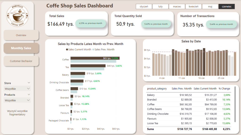
1. Overview

2. Monthy Sales
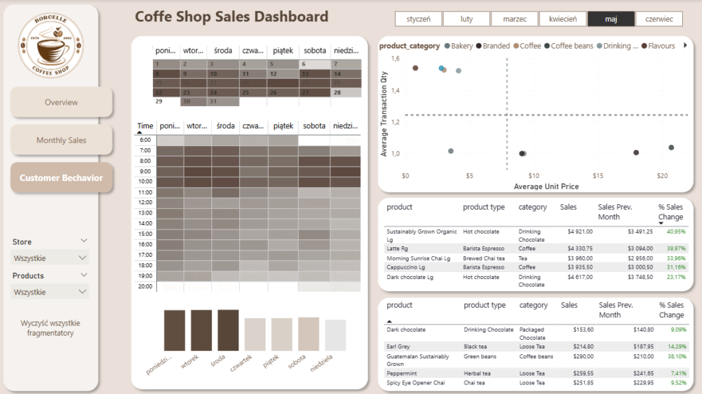
3. Customer Behaviour
Data Cleaning
1.DataFrame

2.Dataset information
Data columns (total 11 columns):
 #   Column            Non-Null Count   Dtype
---  ------            --------------   -----
 0   transaction_id    149116 non-null  int64
 1   transaction_date  149116 non-null  object
 2   transaction_time  149116 non-null  object
 3   transaction_qty   149116 non-null  int64
 4   store_id          149116 non-null  int64
 5   store_location    149116 non-null  object
 6   product_id        149116 non-null  int64
 7   unit_price        149116 non-null  float64
 8   product_category  149116 non-null  object
 9   product_type      149116 non-null  object
 10  product_detail    149116 non-null  object
dtypes: float64(1), int64(4), object(6)
Optimized View for Power BI: Data Transformation and Cleansing in BigQuery
In this SQL snippet, we’re preparing a final dataset for Power BI. Our main objectives include:
- Format Conversions – We utilize functions like
PARSE_DATE,DATETIME, andTIMESTAMPto ensure consistent date and time formats. - Standardization and Calculations – We create a new column (
total_sales) on the fly, calculated from existing fields to streamline subsequent analysis. - Simplified Structure – We limit ourselves to essential columns (e.g.,
transaction_id,store_location,product_category) to make data import and processing in Power BI as efficient as possible.
SELECT
  transaction_id,
  PARSE_DATE('%d.%m.%Y', TRIM(transaction_date)) AS date,
  transaction_time,
  DATETIME(PARSE_DATE('%d.%m.%Y', TRIM(transaction_date)), transaction_time) AS datetime,
  TIMESTAMP(DATETIME(PARSE_DATE('%d.%m.%Y', TRIM(transaction_date)), transaction_time)) AS timestamp,
  transaction_qty,
  store_id,
  store_location,
  product_id,
  unit_price,
  product_category,
  product_type,
  product_detail,
  transaction_qty * unit_price AS total_sales
FROM `coffeshop-447917.coffeshop.PBI_Coffe_Shop`
Dashboard Creation with DAX: Examples and Use Cases
Below are several DAX examples commonly used in Power BI dashboards for time-based analysis, dynamic text display, and custom sorting. Each measure or table creation helps transform raw data into interactive visual insights.
-- Calculates the total sales for the previous month
Sales Prev. Month =
CALCULATE(
    SUM(stg_PBI_Coffe_Shop[total_sales]),
    DATEADD(DateTable[Date], -1, MONTH)
)

-- Formats the transaction change percentage into a readable text format
Button_Transactions =
FORMAT([% Number of Transactions Change], "0.00%") & " vs. previous month"

-- Calculates the percentage of total sales for each product category
GT % Sales =
DIVIDE(
    SUM(stg_PBI_Coffe_Shop[total_sales]),
    CALCULATE(SUM(stg_PBI_Coffe_Shop[total_sales]), ALL(stg_PBI_Coffe_Shop[product_category]))
)

-- Assigns a numeric order to weekdays for correct sorting in visualizations
DaySortOrder =
SWITCH(
    'stg_PBI_Coffe_Shop'[DayOfWeek2],
    "poniedziałek", 1,
    "wtorek", 2,
    "środa", 3,
    "czwartek", 4,
    "piątek", 5,
    "sobota", 6,
    "niedziela", 7
)

-- Calculates the percentage change in sales between the current and previous month
% Sales Change =
DIVIDE(
    [Sales Current Month] - [Sales Prev. Month],
    [Sales Prev. Month],
    0
)

-- Creates a table with predefined sorting order for weekdays
DaySortTable =
DATATABLE(
    "DayOfWeek", STRING,
    "DaySortOrder", INTEGER,
    {
        {"poniedziałek", 1},
        {"wtorek", 2},
        {"środa", 3},
        {"czwartek", 4},
        {"piątek", 5},
        {"sobota", 6},
        {"niedziela", 7}
    }
)

-- Creates a Date Table with additional columns for better time intelligence calculations
DateTable =
ADDCOLUMNS(
    CALENDAR(MIN(stg_PBI_Coffe_Shop[date]), MAX(stg_PBI_Coffe_Shop[date])),
    "Year", YEAR([Date]),
    "Month", MONTH([Date]),
    "MonthName", FORMAT([Date], "MMMM"),
    "YearMonth", FORMAT([Date], "YYYY-MM")
)
Exploratory Data Analysis (EDA) on Coffe Shop Sales
1.Sales Trends Across Time

- Monthly Growth: Sales have shown consistent growth starting in February, indicating either seasonal demand shifts or effective promotional efforts at the beginning of the year.
- End-of-Month Spikes: There’s a subtle but noticeable increase in sales at the end of each month, likely tied to paydays when customers have more disposable income.
- Daily Trends: Sales remain relatively stable throughout the week, with no single day standing out as significantly stronger or weaker.
2. Store Performance
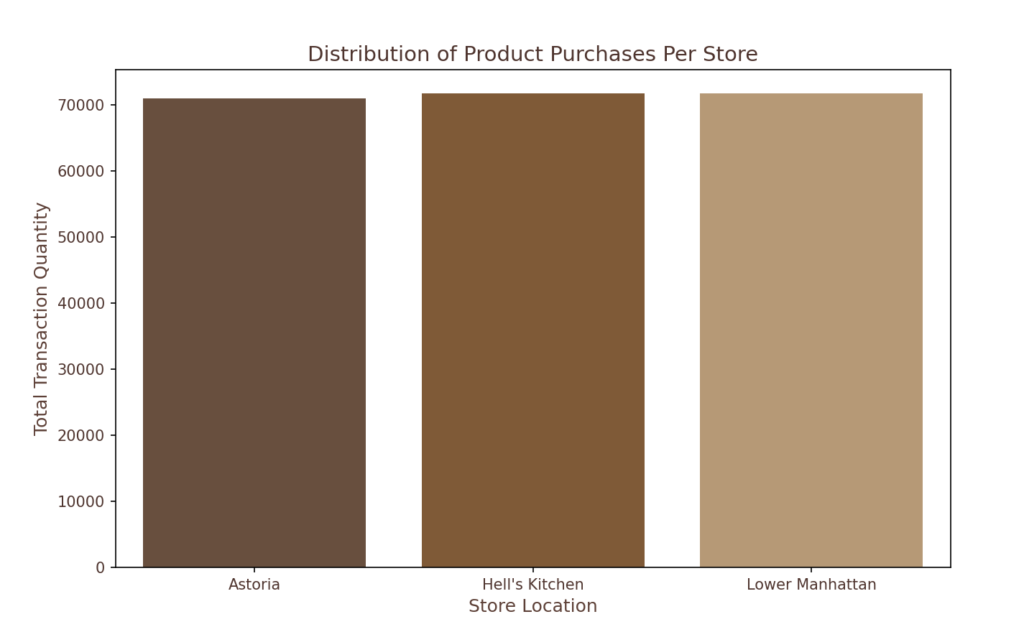
- Balanced Sales Across Locations: All store locations exhibit similar sales performance, meaning that demand is evenly distributed rather than concentrated in any one branch.
4.Purchase Volume Trends and Buying Patterns
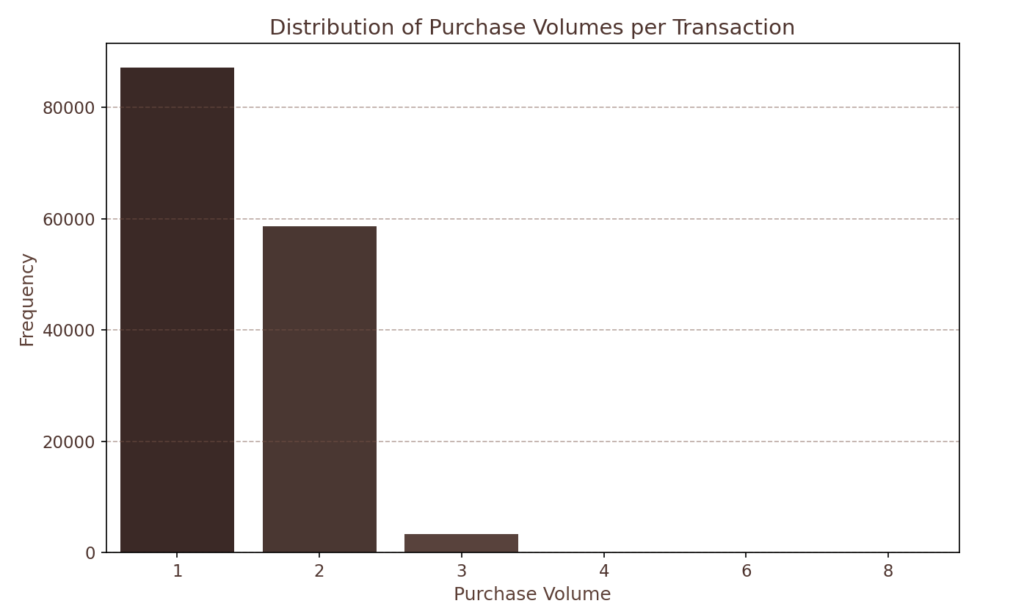
- Single-Item Purchases Lead the Market :The majority of transactions consist of just one or two items, showing a strong preference for quick, on-the-go purchases rather than bulk buying.
- Higher Purchase Volumes Are Rare – Transactions involving three or more items are significantly lower in frequency, suggesting that customers primarily visit for individual consumption rather than group orders or bulk purchases.
- Potential for Higher Ticket Sizes – Since most purchases are minimal, there is an opportunity to encourage customers to buy more through strategic pricing and promotions.
5.Product Category Insights
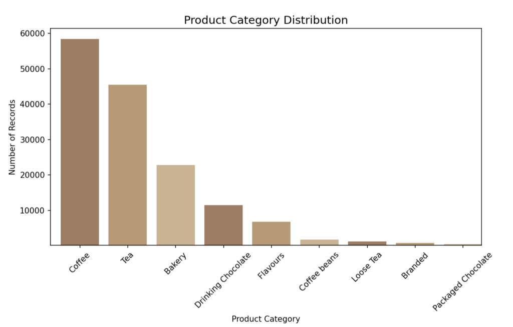
- Most Valuable Porducts (MVP): Coffe and Tea account for nearly 70% of all purchases, making them the primary revenue drivers.
- Premium Products Struggle to Sell: High-end items such as packaged chocolate, branded goods, and coffee beans collectively contribute just 2.8% of total sales, meaning that they are either too expensive or lack strong customer appeal.
6.Customer Behavior
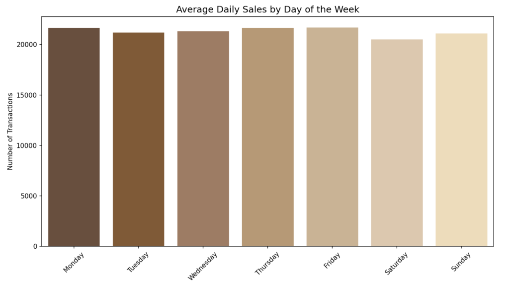
- The sales appear to vary only very slightly over different days of the week as well. There are no visible opportunities to capitalize on.
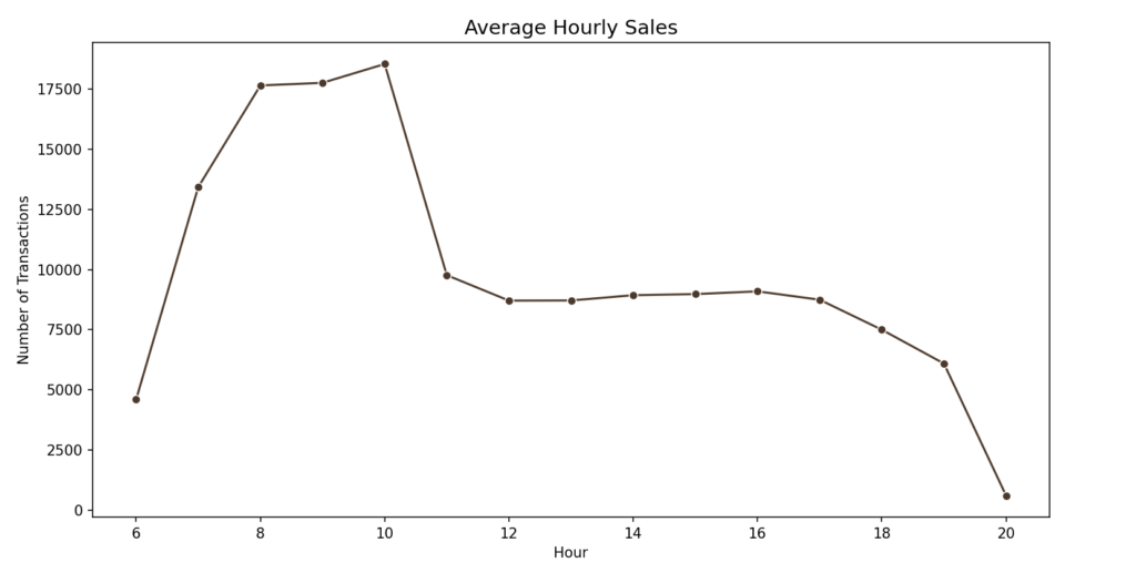
- Peak Hours: The busiest time for transactions is between 8:00 AM and 10:00 AM, aligning with morning routines when customers stop for coffee on their way to work.
- Steady Midday Activity: Sales remain moderate from 11:00 AM to 7:00 PM, which presents an opportunity for promotions aimed at lunchtime and afternoon customers.
Summary of the Exploration
- Store Performance Consistency – Sales and transactions remain relatively uniform across all store locations, indicating a balanced customer distribution.
- Buying Behavior Trends – Most customers purchase only one or two items per transaction, highlighting a preference for quick, individual purchases.
- Dominance of Coffee and Tea – These two categories account for nearly 70% of all sales, reinforcing their position as the most popular offerings.
- Limited Demand for High-Priced Items – The most expensive products represent just 2.8% of total sales, suggesting a lower customer inclination toward premium-priced options.
- Steady Sales Trends – Sales and transaction trends remain largely stable over time, with predictable fluctuations throughout the month.
- Cyclical Patterns in Sales Per Transaction – A noticeable increase in the number of items purchased per transaction is observed toward the end of each month.
- No Significant Variations in Daily Sales – Sales levels remain fairly consistent across different days of the week, with no particular weekday outperforming the others.
- Peak Sales Hours – Sales volume surges between 8 AM and 10 AM, indicating a high morning demand, while activity slows but remains steady from 11 AM to 7 PM.
- Category Preferences Across Stores – There is no major difference in category preferences across store locations, suggesting that product demand is similar regardless of the branch.
Strategic Recommendations
- Optimizing High-Priced Item Sales – Since the most expensive items have lower demand, businesses can explore strategic promotions, limited-time offers, or bundling them with popular products to encourage more purchases.
- Encouraging Larger Transactions – Given that most transactions involve one or two items, sales can be boosted through multi-item promotions, combo deals, or upselling strategies.
- Leveraging Peak Hours for Maximum Revenue – The busiest period between 8 AM and 10 AM presents a key opportunity for premium pricing, exclusive morning specials, or priority service offerings.
- Maximizing Sales During Moderate Hours – The moderate activity from 11 AM to 7 PM can be optimized through afternoon deals, happy-hour discounts, and limited-time seasonal offerings.
- Aligning Staffing with Customer Traffic – The peak morning rush and steady flow throughout the afternoon suggest an opportunity for optimizing employee shifts, ensuring efficient service without overstaffing.